AI-2022spring
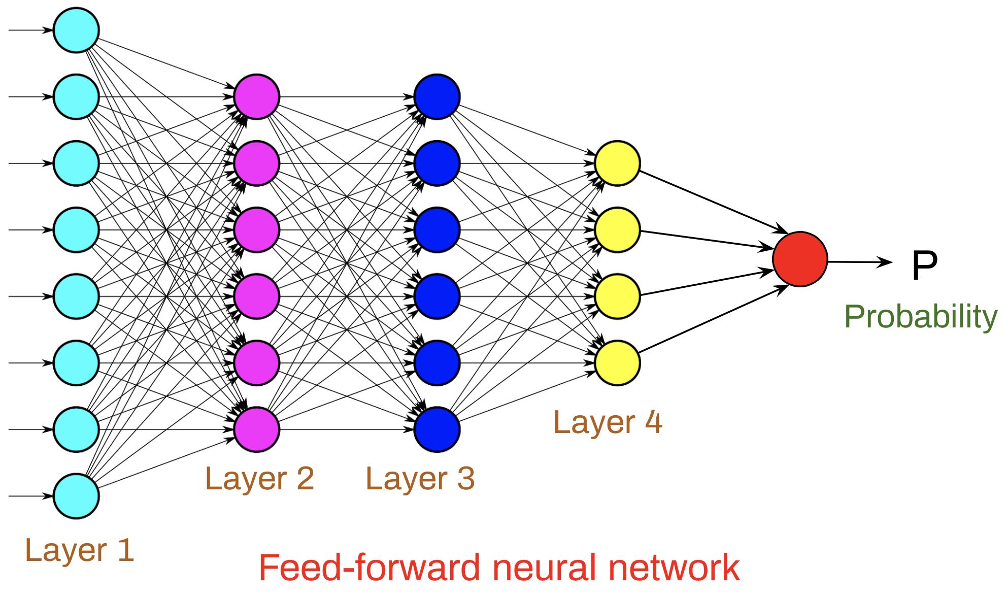
A hands-on introduction to feed-forward neural networks using Tensorflow and Keras
This is a mini crash course on using Tensorflow to develop feed-forward neural networks. It contains 10 scaffolded activities. If you already have some background in Tensorflow, Keras, and/or machine learning, you may also be interested to take the machine learning crash course that Google recently released. You may also find it helpful to often refer to this recipe for supervised learning development.
Activity 1: Practice Python3
In this activity, the task is to learn how to use Google Colab and practice Python3. If you are doing Python programming for the first time, please practice Python3 at online platforms such as codewars.org too. If you fear learning new things (including Python3) you are welcome to take the Learning How to Learn course, the world’s most popular online course.
- Lectures: Google Colab and Python3
- Notebooks: Python3
- Alternatives to Google Colab: Kaggle Notebooks, PyCharm with a .edu account, Local Installation
Activity 2: Practice Numpy, Matplotlib, and Pandas
In this activity, the task is to practice Numpy, Matplotlib, Plotly, Pandas for basic data analysis, and techniques of data cleaning and data normalization.
- Lectures: Numpy, Matplotlib & Plotly, Data normalization, and Data cleaning
- Notebooks: Numpy, Matplotlib & Plotly, Pandas, and Normalization techniques
- Reading: Ordinal and One-Hot Encodings for Categorical Data
For the remaining activities below please clean and use the Pima diabetes dataset, the Wine quality dataset, and one additional dataset of your choice. Please practice using at least two/three datasets.
Activity 3: Logistic regression
In this activity, the goal is to practice logistic regression on a dataset with more than one input variables. When selecting a variable (column) for performing logistic regression, it is important to select a binary variable as the output variable. In other words, the values of this variable must be a 0 or a 1, nothing else. Before feeding the data to the model, it is often important to normalize/standardize your input dataset. You may need to normalize your data for classification to work. Here, the task is to perform logistic regression on your classification dataset.
- Lectures: Logistic regression and Data normalization
- Notebook: Logistic regression
Metrics for evaluating a binary classification model:
- Accuracy, precision, recall, F1-score
- ROC curve and area under the curve (AUC)
Metrics for evaluating a regression model:
- MAE, MSE
- Residuals
- True vs prediction scatter plot
- Pearson’s correlation coefficient
Activity 4: Binary classification using neural networks
In this activity, the goal is to practice training a neural network model to perform binary classification. A neural network classifier should be more accurate than a basic logistic regression model. This is because a neural network model has more parameters (weights and biases) to learn the patterns in the data. A binary classifier can be evaluated using metrics such as accuracy, precision, and recall. Interpreting the accuracy of a binary classifier can be tricky. This is because the baseline accuracy, i.e., minimum accuracy, is at least 50%. Please note that every dataset has its own baseline. You will need to find the baseline accuracy for your dataset by calculating the percentage of positive or negative labels (whichever is higher). A good classifier should result in an accuracy that is much higher than a baseline accuracy. The tasks in this activity are (i) Build a neural network classifier for your dataset, (ii) Evaluate your model using accuracy, precision, and recall, (iii) Compare the accuracy of your model with the baseline accuracy, and (iv) Compare the performance of the neural network with a logistic regression model.
- Lectures: Binary classification
- Articles: A Visual and Interactive Guide to the Basics of Neural Networks
- Notebook: Binary classification | Wine quality dataset
Activity 5: Overfitting vs generalization
In this activity, the goal is to learn the concepts of overfitting, underfitting, generalization, and the purpose of splitting a dataset into training set and validation set. For a standard tabular classification dataset of your choice, where the output variable is a binary variable, the first step is to shuffle the rows (see example code below). The next step is to split the rows into training and validation set. For small datasets, selecting a random 30% of the rows as the validation set and leaving the rest as the training set works well. For larger datasets, smaller percents can be enough. This splitting yeilds four numpy arrays - XTRAIN, YTRAIN, XVALID, and YVALID (see example code below). For normalizing the data and to obtain the ‘mean’ and ‘standard deviation’ it is important to only use the XTRAIN array, not XVALID. XVALID should be normalized using the mean and standard deviation obtained from XTRAIN. Then the main question one should ask is - if a model is trained using the training data (XTRAIN and YTRAIN) how does it perform on the validation set (XVALID and YVALID)? In this activity there are two tasks: (i) Build a neural network model to overfit the training set (to get almost 100% accuracy or as high as it is possible) and then evaluate on the validation set, and (ii) Evaluate the accuracy of the model for the training set and the validation set and discuss your findings. To obtain high accuracy on the training set, one can build a larger neural network (with more layers and more neurons per layer) and train as long as possible.
# Shuffle the datasets
import random
np.random.shuffle(dataset)
# Split into training and validation, 30% validation set and 70% training
index_30percent = int(0.3 * len(dataset[:, 0]))
print(index_30percent)
XVALID = dataset[:index_30percent, "all input columns"]
YVALID = dataset[:index_30percent, "output column"]
XTRAIN = dataset[index_30percent:, "all input columns"]
YTRAIN = dataset[index_30percent:, "output column"]
# Learn the model from training set
model.fit(XTRAIN, YTRAIN, ...)
# Evaluate on the training set (should deliver high accuracy)
P = model.predict(XTRAIN)
accuracy = model.evaluate(XTRAIN, YTRAIN)
#Evaluate on the validation set
P = model.predict(XVALID)
accuracy = model.evaluate(XVALID, YVALID)
In the notebook where you practice, also answer the following:
- Does your model perform better (in terms of accuracy) on the training set or validation set? Is this a problem? How to avoid this problem?
- Why can over training be a problem?
- What is the difference between generalization, overfitting, and underfitting?
- Why should you not normalize XVALID separately, i.e. why should we use the parameters from XTRAIN to normalize XVALID?
Activity 6: Learning curves
This activity assumes that you have successfully completed all previous activities. It also requires some focus. Learning curves are a key to debug and diagnose a model’s performance. The goal in this activity is to plot learning curves and to interpret various learning curves. For a regression dataset of your choice, the first step is to shuffle the dataset. The next step is to split the dataset into the four arrays: XTRAIN, YTRAIN, XVALID, and YVALID. The next step is to train a neural network model using model.fit(). However, this time, XVALID and YVALID will also be passed as arguments to the model.fit() method. This is so when we call the method, it can evaluate the model on the validation set at the end of each epoch (see code block below). It is crucial to understand that the model.fit() method does NOT use the validation dataset to perform the learning, it is only to evaluate the model after each epoch. When calling the model.fit() method we can also save its output in a variable, usually named history. This variable can be used to plot learning curves (see code block below). The task in this activity is to plot many learning curves in various scenarios. In particular, it is of interest to observe and analyze how the learning plots look like in various settings. The following article discusses learning curves in more detail.
- Lectures: Some insights on learning curves
- Articles: Learning curves for diagnosing machine learning model performance
# Do the training (specify the validation set as well)
history = model.fit(XTRAIN, YTRAIN, validation_data = (XVALID, YVALID), verbose = 1)
# Check what's in the history
print(history.params)
# Plot the learning curves (loss/accuracy/MAE)
plt.plot(history.history['accuracy']) # replace with accuracy/MAE
plt.plot(history.history['val_accuracy']) # replace with val_accuracy, etc.
plt.ylabel('Accuracy')
plt.xlabel('epoch')
plt.legend(['training data', 'validation data'], loc='lower right')
plt.show()
Produce learning curves that represent the following cases:
- the validation set is too small relative to the training set - for example, only 1% or 2% of the total rows of data.
- the training set is too small compared to the validation sat - for example, only 1% or 2% of the total rows of data.
- a good learning curve (practically good)
- an overfitting model
- a model that shows that further training is required
- an underfit model that does not have sufficient capacity (also may imply that the data itself is difficult)
Activity 7: Fine-tuning hyper-parameters of your model
In this activity, the task is to learn how to design and train a model that does well on the unseen (validation) dataset. The weights and biases of a neural network model are its parameters. The parameters such as the number of layers of neurons, numbers of neurons in each layer, number of epochs, batch size, activation functions, choice of optimizer, choice of loss function, etc. are the hyperparameters of a model. When training a model for a new dataset a crucial question is - what combinations of hyperameters yield the maximum accuracy on the validation set? Remember, when playing with activation functions, the activation of the last layer should not change - it should always be sigmoid for binary classification and ReLU or linear for regression. The task in this activity is to try as many hyperparameters as possible to obtain the highest possible accuracy on the validation set. For a classification dataset of your choice, the first step is to create a notebook where you can train the model using the training set and evaluate on the validation set. Then, the objective is to find the optimal (best) hyper-parameters that maximize the accuracy (or minimize MAE) on the validation set.
Below are the hyperparameters to optimize:
- The number of layers in the neural network (try 1, 2, 4, 8, 16, etc.).
- The number of neurons in each layer (try 2, 4, 8, 16, 32, 64, 128, 256, 512, etc.).
- Various batch sizes (8, 16, 32, 64, etc.).
- Various number of epochs (2, 4, 8, …, 5000, etc.).
- Various optimizers (rmsprop, sgd, nadam, adam, gd, etc.)
- Various activation functions for the intermediate layers (relu, sigmoid, elu, etc.)
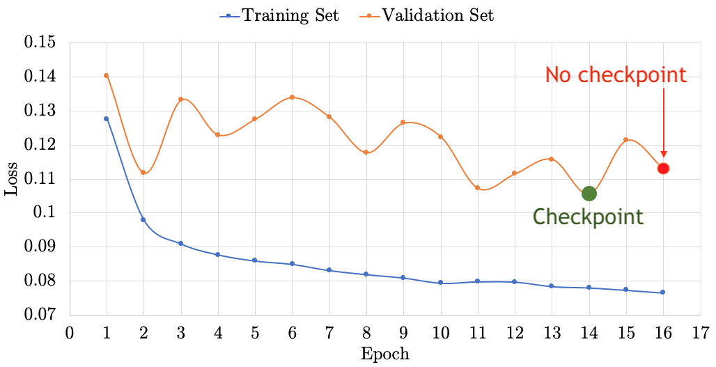
Activity 8: Early stopping
Assumption: You already know (tentatively) what hyperparameters are good for your dataset
- Find a regression dataset of your choice and split into training and validation set
- There are two objectives in this activity:
a. Implement automatic stopping of training if the accuracy does not improve for certain epochs
b. Implement automatic saving of the best model (best on the validation set) - Define callbacks as follows (and fix the obvious bugs):
from tensorflow.keras.callbacks import EarlyStopping, ModelCheckpoint # File name must be in quotes callback_a = ModelCheckpoint(filepath = your_model.hdf5, monitor='val_loss', save_best_only = True, save_weights_only = True, verbose = 1) # The patience value can be 10, 20, 100, etc. depending on when your model starts to overfit callback_b = EarlyStopping(monitor='val_loss', mode='min', patience=your_patience_value, verbose=1) - Update your
model.fit()by adding the callbacks:history = model.fit(XTRAIN, YTRAIN, validation_data=(XVALID, YVALID), epochs=?, batch_size=?, callbacks = [callback_a, callback_b]) - Before you evaluate your model on the validation set, it is important to load the “checkpoint-ed” model:
# File name must be in quotes model.load_weights(your_model.hdf5) - Plot the learning curves and demonstrate that model checkpointing helps to obtain higher accuracy on the validation set
- At the end of your notebook, answer the following questions:
a. Almost always, training with early stopping finishes faster (because it stops early). Approximately, how long does it take for your training to finish with and without early stopping?
b. When model checkpointing, your checkpointed model will almost always be more accurate on the validation set. What is the MAE on the Validation set with and without model checkpointing?
Activity 9: Iterative feature removal & selection
So far, it is assumed that given a dataset (of your choice) you can build a model that can do reasonably well on the validation set, i.e. you have a good idea of the network architecture needed, the number of epochs needed, model Checkpointing, the approximate MAE or accuracy that one might expect, etc. In this activity you will implement a simple Recursive Feature Elimination (RFE) technique to remove redundant or insignificant input features. Here are the steps involved:
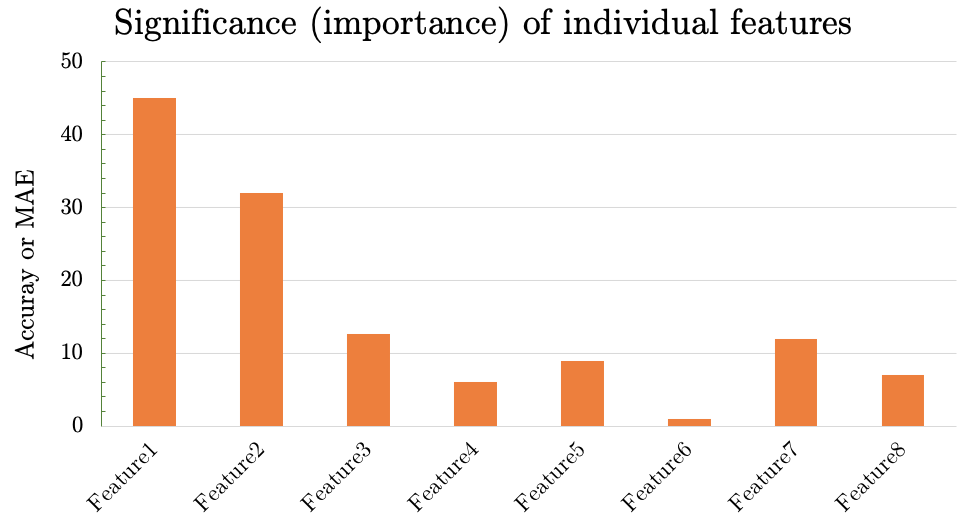
- If you have 10 input features/columns, train 10 models where each model only receives one feature at a time. For example, if age, BMI, and blood pressure are your only three input features, you train three models: one that only take age as input, another that only takes BMI as the input, and the last one that takes only blood pressure as the input. The validation accuracy of these three models will indicate the relative importance of the three features. You should plot these validation accuracies in the form of a bar diagram. If all your accuracies are more than 80%, your plot’s y-axis should be limited to 80-100.
- Expected output 1: Plot the significance (importance) of each feature after training your model using one feature at a time:
a. X-axis represents the feature that was used as the input
b. Y-axis is accuracy or MAE of the validation set
- Expected output 1: Plot the significance (importance) of each feature after training your model using one feature at a time:
- From the previous step you have the significance/important of each feature. The feature that yields the highest accuray is the most important feature. Observing these MAE/accuracy values, we can rank the features by their importance (how informative each one is).
- Starting with the most unimportant feature, remove one feature at a time (without replacement) and train various models. You can iteratively repeat the process removing more and more unimportant features. For example, if BMI is the most important feature and blood pressure is the least important one, you would train two models: one without blood pressure, and one without blood pressure and age. Plot the validation dataset accuracy of all the models that you tested. The overall objective is to identify non-informative input features and remove them from the dataset. Finally, you can compare your feature-reduced model with the original model with all input features and discuss the difference in accuracy.
- Expected output 2: Plot to report your findings:
a. X-axis represents feature removal, for example, second entry is after removing feature1, and third entry is after removing feature1 and feature2
b. Y-axis is accuracy or MAE of the validation set

- Expected output 2: Plot to report your findings: